5. Singular Value Decomposition (SVD)#
5.1. Overview#
The singular value decomposition (SVD) is a work-horse in applications of least squares projection that form foundations for many statistical and machine learning methods.
After defining the SVD, we’ll describe how it connects to
four fundamental spaces of linear algebra
low-rank approximations of matrices
under-determined and over-determined least squares regressions (see the exercises)
principal components analysis (PCA)
In a sequel to this lecture, VARs and DMDs, we’ll describe how SVDs provide ways rapidly to compute reduced-rank approximations to first-order vector autoregressions (VARs) by means of a dynamic mode decomposition (DMD).
Like principal components analysis, DMD can be thought of as a data-reduction procedure that represents salient patterns by projecting data onto a limited set of factors.
5.2. The setting#
Let \(X\) be an \(m \times n\) matrix of rank \(p\).
Necessarily, \(p \leq \min(m,n)\).
In much of this lecture, we’ll think of \(X\) as a matrix of data in which
each column is an individual – a time period or person, depending on the application
each row is a random variable describing an attribute of a time period or a person, depending on the application
We’ll be interested in two situations
A short and fat case in which \(m \ll n\), so that there are many more columns (individuals) than rows (attributes).
A tall and skinny case in which \(m \gg n\), so that there are many more rows (attributes) than columns (individuals).
We’ll apply a singular value decomposition of \(X\) in both situations.
In the \(m \ll n\) case in which there are many more individuals \(n\) than attributes \(m\), we can calculate sample moments of a joint distribution by taking averages across observations of functions of the observations.
In this \(m \ll n\) case, we’ll look for patterns by using a singular value decomposition to do a principal components analysis (PCA).
In the \(m \gg n\) case in which there are many more attributes \(m\) than individuals \(n\) and when we are in a time-series setting in which \(n\) equals the number of time periods covered in the data set \(X\), we’ll proceed in a different way.
In the sequel VARs and DMDs, we’ll again use a singular value decomposition, but now to construct a dynamic mode decomposition (DMD).
5.3. Singular value decomposition#
A singular value decomposition of an \(m \times n\) matrix \(X\) of rank \(p \leq \min(m,n)\) is
where
and
\(U\) is an \(m \times m\) orthogonal matrix of left singular vectors of \(X\)
Columns of \(U\) are eigenvectors of \(X X^\top \)
\(V\) is an \(n \times n\) orthogonal matrix of right singular vectors of \(X\)
Columns of \(V\) are eigenvectors of \(X^\top X\)
\(\Sigma\) is an \(m \times n\) matrix in which the first \(p\) places on its main diagonal are positive numbers \(\sigma_1 \geq \sigma_2 \geq \cdots \geq \sigma_p\) called singular values; remaining entries of \(\Sigma\) are all zero
The \(p\) singular values are positive square roots of the nonzero eigenvalues of the \(m \times m\) matrix \(X X^\top \) and also of the \(n \times n\) matrix \(X^\top X\)
We adopt a convention that when \(U\) is a complex valued matrix, \(U^\top \) denotes the conjugate-transpose or Hermitian-transpose of \(U\), meaning that \(U_{ij}^\top \) is the complex conjugate of \(U_{ji}\).
Similarly, when \(V\) is a complex valued matrix, \(V^\top \) denotes the conjugate-transpose or Hermitian-transpose of \(V\)
The matrices \(U,\Sigma,V\) entail linear transformations that reshape vectors in the following ways:
multiplying vectors by the unitary matrices \(U\) and \(V\) rotates them, but leaves angles between vectors and lengths of vectors unchanged.
multiplying vectors by the diagonal matrix \(\Sigma\) rescales each coordinate by a singular value (and adds or drops coordinates when \(m \neq n\)); in general this changes both lengths of vectors and angles between them.
Thus, representation (5.1) asserts that multiplying an \(n \times 1\) vector \(y\) by the \(m \times n\) matrix \(X\) amounts to performing the following three multiplications of \(y\) sequentially:
rotating \(y\) by computing \(V^\top y\)
rescaling \(V^\top y\) by multiplying it by \(\Sigma\)
rotating \(\Sigma V^\top y\) by multiplying it by \(U\)
This structure of the \(m \times n\) matrix \(X\) opens the door to constructing systems of data encoders and decoders.
Thus,
\(V^\top\) is an encoder
\(\Sigma\) is an operator to be applied to the encoded data
\(U\) is a decoder to be applied to the output from applying operator \(\Sigma\) to the encoded data
We’ll apply this circle of ideas in the sequel VARs and DMDs when we study dynamic mode decompositions.
Road ahead
What we have described above is called a full SVD.
In a full SVD, the shapes of \(U\), \(\Sigma\), and \(V\) are \(\left(m, m\right)\), \(\left(m, n\right)\), \(\left(n, n\right)\), respectively.
Later we’ll also describe an economy or reduced SVD.
Before we study a reduced SVD we’ll say a little more about properties of a full SVD.
5.4. Four fundamental subspaces#
Let \({\mathcal C}\) denote a column space, \({\mathcal N}\) denote a null space, and \({\mathcal R}\) denote a row space.
Let’s start by recalling the four fundamental subspaces of an \(m \times n\) matrix \(X\) of rank \(p\).
The column space of \(X\), denoted \({\mathcal C}(X)\), is the span of the columns of \(X\), i.e., all vectors \(y\) that can be written as linear combinations of columns of \(X\). Its dimension is \(p\).
The null space of \(X\), denoted \({\mathcal N}(X)\) consists of all vectors \(y\) that satisfy \(X y = 0\). Its dimension is \(n-p\).
The row space of \(X\), denoted \({\mathcal R}(X)\) is the column space of \(X^\top \). It consists of all vectors \(z\) that can be written as linear combinations of rows of \(X\). Its dimension is \(p\).
The left null space of \(X\), denoted \({\mathcal N}(X^\top )\), consists of all vectors \(z\) such that \(X^\top z =0\). Its dimension is \(m-p\).
For a full SVD of a matrix \(X\), the matrix \(U\) of left singular vectors and the matrix \(V\) of right singular vectors contain orthogonal bases for all four subspaces.
They form two pairs of orthogonal subspaces that we’ll describe now.
Let \(u_i, i = 1, \ldots, m\) be the \(m\) column vectors of \(U\) and let \(v_i, i = 1, \ldots, n\) be the \(n\) column vectors of \(V\).
Let’s write the full SVD of \(X\) as
where \(\Sigma_p\) is a \(p \times p\) diagonal matrix with the \(p\) singular values on the diagonal and
Representation (5.2) implies that
or
or
Equations (5.4) tell how the transformation \(X\) maps a pair of orthonormal vectors \(v_i, v_j\) for \(i\) and \(j\) both less than or equal to the rank \(p\) of \(X\) into a pair of orthogonal vectors \(\sigma_i u_i, \sigma_j u_j\) with lengths \(\sigma_i\) and \(\sigma_j\).
Equations (5.3) assert that
Taking transposes on both sides of representation (5.2) implies
or
or
Notice how equations (5.6) assert that the transformation \(X^\top \) maps a pair of distinct orthonormal vectors \(u_i, u_j\) for \(i\) and \(j\) both less than or equal to the rank \(p\) of \(X\) into a pair of orthogonal vectors \(\sigma_i v_i, \sigma_j v_j\).
Equations (5.5) assert that
Thus, taken together, the systems of equations (5.3) and (5.5) describe the four fundamental subspaces of \(X\) in the following ways:
Since \(U\) and \(V\) are both orthonormal matrices, collection (5.7) asserts that
\(U_L\) is an orthonormal basis for the column space of \(X\)
\(U_R\) is an orthonormal basis for the null space of \(X^\top \)
\(V_L\) is an orthonormal basis for the row space of \(X\)
\(V_R\) is an orthonormal basis for the null space of \(X\)
We have verified the four claims in (5.7) simply by performing the multiplications called for by the right side of (5.2) and reading them.
The claims in (5.7) and the fact that \(U\) and \(V\) are both unitary (i.e., orthonormal) matrices imply that
the column space of \(X\) is orthogonal to the null space of \(X^\top \)
the null space of \(X\) is orthogonal to the row space of \(X\)
Sometimes these properties are described with the following two pairs of orthogonal complement subspaces:
\({\mathcal C}(X)\) is the orthogonal complement of \({\mathcal N}(X^\top )\)
\({\mathcal R}(X)\) is the orthogonal complement of \({\mathcal N}(X)\)
Let’s do an example.
import numpy as np
import numpy.linalg as LA
import matplotlib.pyplot as plt

rng = np.random.default_rng(1234)
Having imported these modules, let’s do the example.
We use a \(4 \times 5\) matrix of rank \(2\), so that the four subspaces have dimensions \(2\), \(2\), \(2\), and \(3\).
Note that np.linalg.svd returns \(V^\top\), not \(V\), as its third output.
So the row space and the null space are spanned by rows of that output.
np.set_printoptions(precision=2, suppress=True)

# Define the matrix
A = np.array([[1, 2, 3, 4, 5],
              [2, 3, 4, 5, 6],
              [3, 4, 5, 6, 7],
              [4, 5, 6, 7, 8]])

# Compute the SVD of the matrix; the third output is V^T
U, S, VT = np.linalg.svd(A, full_matrices=True)

# Compute the rank of the matrix
rank = np.linalg.matrix_rank(A)

print("Rank of matrix:\n", rank)
print("S: \n", S)

# Orthonormal bases for the four fundamental subspaces
col_space = U[:, :rank]            # C(A),   a subspace of R^4
left_null_space = U[:, rank:]      # N(A^T), a subspace of R^4
row_space = VT[:rank, :].T         # R(A),   a subspace of R^5
null_space = VT[rank:, :].T        # N(A),   a subspace of R^5

print("Column space:\n", col_space)
print("Left null space:\n", left_null_space)
print("Row space:\n", row_space)
print("Null space:\n", null_space)
Rank of matrix:
 2
S:
 [21.63  1.46  0.    0.  ]
Column space:
 [[ 0.34  0.76]
 [ 0.44  0.33]
 [ 0.54 -0.11]
 [ 0.64 -0.54]]
Left null space:
 [[-0.27  0.48]
 [ 0.71 -0.44]
 [-0.62 -0.56]
 [ 0.18  0.52]]
Row space:
 [[ 0.25 -0.73]
 [ 0.34 -0.43]
 [ 0.43 -0.13]
 [ 0.52  0.18]
 [ 0.61  0.48]]
Null space:
 [[ 0.62 -0.08  0.08]
 [-0.71 -0.05  0.45]
 [-0.24 -0.18 -0.84]
 [ 0.11  0.83  0.03]
 [ 0.21 -0.52  0.29]]
Let’s verify that the bases have the properties that (5.7) asserts.
print("A @ null_space = 0:        ", np.allclose(A @ null_space, 0))
print("A.T @ left_null_space = 0: ", np.allclose(A.T @ left_null_space, 0))
print("col_space ⟂ left_null_space:", np.allclose(col_space.T @ left_null_space, 0))
print("row_space ⟂ null_space:    ", np.allclose(row_space.T @ null_space, 0))
A @ null_space = 0:         True
A.T @ left_null_space = 0:  True
col_space ⟂ left_null_space: True
row_space ⟂ null_space:     True
5.5. Eckart-Young theorem#
Suppose that we want to construct the best rank \(r\) approximation of an \(m \times n\) matrix \(X\).
By best, we mean a matrix \(X_r\) of rank \(r < p\) that, among all rank \(r\) matrices of dimension \(m \times n\), minimizes
where \( || \cdot || \) denotes a norm of a matrix.
Three popular matrix norms of an \(m \times n\) matrix \(X\) can be expressed in terms of the singular values of \(X\)
the spectral or \(l^2\) norm \(|| X ||_2 = \max_{||y|| \neq 0} \frac{||X y ||}{||y||} = \sigma_1\)
the Frobenius norm \(||X ||_F = \sqrt{\sigma_1^2 + \cdots + \sigma_p^2}\)
the nuclear norm \( || X ||_N = \sigma_1 + \cdots + \sigma_p \)
The Eckart-Young theorem states that for each of these three norms, the same rank \(r\) matrix is best and that it equals
where \(U_r\) and \(V_r\) consist of the first \(r\) columns of \(U\) and \(V\), respectively, and \(\Sigma_r\) is the \(r \times r\) diagonal matrix of the \(r\) largest singular values.
The resulting approximation errors are
This is a very powerful theorem.
It says that we can approximate an \(m \times n\) matrix \(X\) of rank \(p\) by an \(m \times n\) matrix of rank \(r < p\) built from the \(r\) largest singular values of \(X\) and their singular vectors, and that the singular values that we discard measure the approximation error.
If a few singular values are much larger than the others, a low-rank approximation captures most of \(X\) while requiring us to store only \(r(m + n + 1)\) numbers instead of \(mn\).
You can read about the Eckart-Young theorem and some of its uses here.
We’ll make use of this theorem when we discuss principal components analysis (PCA) below.
It also underlies the sequel VARs and DMDs, where the pseudo-inverse
of the approximation \(\hat X_r\) is a key ingredient of a dynamic mode decomposition.
Exercise 5.2 and Exercise 5.3 explore these ideas.
5.6. Full and reduced SVD’s#
Up to now we have described properties of a full SVD in which shapes of \(U\), \(\Sigma\), and \(V\) are \(\left(m, m\right)\), \(\left(m, n\right)\), \(\left(n, n\right)\), respectively.
There is an alternative bookkeeping convention called an economy or reduced SVD in which the shapes of \(U, \Sigma\) and \(V\) are different from what they are in a full SVD.
Because we assume that \(X\) has rank \(p\), there are only \(p\) nonzero singular values, where \(p=\textrm{rank}(X)\leq\min\left(m, n\right)\).
A reduced SVD uses this fact to express \(U\), \(\Sigma\), and \(V\) as matrices with shapes \(\left(m, p\right)\), \(\left(p, p\right)\), \(\left( n, p\right)\).
You can read about reduced and full SVD here https://numpy.org/doc/stable/reference/generated/numpy.linalg.svd.html
(With the option full_matrices=False, numpy returns \(\min(m, n)\) columns of \(U\) and \(V\); when \(p < \min(m,n)\), we drop the columns that correspond to zero singular values to obtain a reduced SVD in the sense used here.)
For a full SVD,
But not all these properties hold for a reduced SVD.
For a reduced SVD, \(U^\top U = I_{p \times p}\) and \(V^\top V = I_{p \times p}\) always hold, but \(U U^\top = I_{m \times m}\) holds only if \(p = m\) and \(V V^\top = I_{n \times n}\) holds only if \(p = n\).
Which properties hold thus depends on whether we are in a tall-skinny case or a short-fat case.
In a tall-skinny case in which \(m \gg n\) and \(X\) has full column rank \(p = n\), for a reduced SVD
In a short-fat case in which \(m \ll n\) and \(X\) has full row rank \(p = m\), for a reduced SVD
When we study dynamic mode decompositions in the sequel VARs and DMDs, we shall want to remember these properties because we will use a reduced SVD in a tall-skinny case.
Let’s do an example to compare full and reduced SVD’s.
To review,
in a full SVD
\(U\) is \(m \times m\)
\(\Sigma\) is \(m \times n\)
\(V\) is \(n \times n\)
in a reduced SVD
\(U\) is \(m \times p\)
\(\Sigma\) is \(p\times p\)
\(V\) is \(n \times p\)
First, let’s study a case in which \(m = 5 > n = 2\).
(This is a small example of the tall-skinny case that will concern us when we study dynamic mode decompositions in the sequel.)
X = rng.random((5, 2))
U, S, V = np.linalg.svd(X, full_matrices=True)  # full SVD
Uhat, Shat, Vhat = np.linalg.svd(X, full_matrices=False) # economy SVD
print('U, S, V =')
U, S, V
U, S, V =
(array([[-0.58,  0.17, -0.2 , -0.67, -0.38],
        [-0.53, -0.23, -0.05,  0.68, -0.45],
        [-0.19,  0.03,  0.98, -0.09, -0.04],
        [-0.18,  0.92, -0.03,  0.29,  0.19],
        [-0.55, -0.27, -0.07, -0.01,  0.78]]),
 array([1.8 , 0.24]),
 array([[-0.95, -0.33],
        [-0.33,  0.95]]))
print('Uhat, Shat, Vhat = ')
Uhat, Shat, Vhat
Uhat, Shat, Vhat =
(array([[-0.58,  0.17],
        [-0.53, -0.23],
        [-0.19,  0.03],
        [-0.18,  0.92],
        [-0.55, -0.27]]),
 array([1.8 , 0.24]),
 array([[-0.95, -0.33],
        [-0.33,  0.95]]))
rr = np.linalg.matrix_rank(X)
print(f'rank of X = {rr}')
rank of X = 2
Properties:
Where \(U\) is constructed via a full SVD, \(U^\top U = I_{m\times m}\) and \(U U^\top = I_{m \times m}\)
Where \(\hat U\) is constructed via a reduced SVD, although \(\hat U^\top \hat U = I_{p\times p}\), it happens that \(\hat U \hat U^\top \neq I_{m \times m}\)
We illustrate these properties for our example with the following code cells.
UTU = U.T@U
UUT = U@U.T
print('UUT, UTU = ')
UUT, UTU
UUT, UTU =
(array([[ 1.,  0., -0., -0., -0.],
        [ 0.,  1., -0.,  0., -0.],
        [-0., -0.,  1., -0., -0.],
        [-0.,  0., -0.,  1.,  0.],
        [-0., -0., -0.,  0.,  1.]]),
 array([[ 1., -0., -0.,  0., -0.],
        [-0.,  1., -0.,  0., -0.],
        [-0., -0.,  1.,  0., -0.],
        [ 0.,  0.,  0.,  1.,  0.],
        [-0., -0., -0.,  0.,  1.]]))
UhatUhatT = Uhat@Uhat.T
UhatTUhat = Uhat.T@Uhat
print('UhatUhatT, UhatTUhat= ')
UhatUhatT, UhatTUhat
UhatUhatT, UhatTUhat=
(array([[ 0.37,  0.27,  0.12,  0.26,  0.28],
        [ 0.27,  0.33,  0.09, -0.11,  0.36],
        [ 0.12,  0.09,  0.04,  0.06,  0.1 ],
        [ 0.26, -0.11,  0.06,  0.88, -0.15],
        [ 0.28,  0.36,  0.1 , -0.15,  0.38]]),
 array([[ 1., -0.],
        [-0.,  1.]]))
Remarks:
The cells above illustrate the application of the full_matrices=True and full_matrices=False options.
Using full_matrices=False returns a reduced singular value decomposition.
The full and reduced SVD’s both accurately decompose an \(m \times n\) matrix \(X\).
When we study dynamic mode decompositions in the sequel, it will be important for us to remember the preceding properties of full and reduced SVD’s in such tall-skinny cases.
Now let’s turn to a short-fat case.
To illustrate this case, we’ll set \(m = 2 < 5 = n\) and compute both full and reduced SVD’s.
X = rng.random((2, 5))
U, S, V = np.linalg.svd(X, full_matrices=True)  # full SVD
Uhat, Shat, Vhat = np.linalg.svd(X, full_matrices=False) # economy SVD
print('U, S, V = ')
U, S, V
U, S, V =
(array([[ 0.78, -0.63],
        [ 0.63,  0.78]]),
 array([1.97, 0.68]),
 array([[ 0.39,  0.48,  0.41,  0.4 ,  0.55],
        [ 0.35,  0.28, -0.55, -0.61,  0.37],
        [-0.52,  0.45,  0.49, -0.54, -0.  ],
        [-0.52,  0.51, -0.54,  0.43,  0.02],
        [-0.44, -0.49, -0.02, -0.  ,  0.75]]))
print('Uhat, Shat, Vhat = ')
Uhat, Shat, Vhat
Uhat, Shat, Vhat =
(array([[ 0.78, -0.63],
        [ 0.63,  0.78]]),
 array([1.97, 0.68]),
 array([[ 0.39,  0.48,  0.41,  0.4 ,  0.55],
        [ 0.35,  0.28, -0.55, -0.61,  0.37]]))
Let’s verify that our reduced SVD accurately represents \(X\)
SShat=np.diag(Shat)
np.allclose(X, Uhat@SShat@Vhat)
True
5.7. Polar decomposition#
A reduced singular value decomposition (SVD) of \(X\) is related to a polar decomposition of \(X\)
where
and in our reduced SVD
\(U\) is an \(m \times p\) orthonormal matrix
\(\Sigma\) is a \(p \times p\) diagonal matrix
\(V\) is an \(n \times p\) orthonormal matrix
Because \(U^\top U = I\), we have \(SQ = U \Sigma U^\top U V^\top = U \Sigma V^\top = X\).
Here
\(S\) is an \(m \times m\) symmetric positive semidefinite matrix
\(Q\) is an \(m \times n\) matrix with \(Q Q^\top = U U^\top\); so when \(p = m\), as for a short-fat \(X\) with full row rank, \(Q Q^\top = I\) and \(Q\) has orthonormal rows
5.8. Application: principal components analysis (PCA)#
Let’s begin with a case in which \(n \gg m\), so that we have many more individuals \(n\) than attributes \(m\).
The matrix \(X\) is short and fat in an \(n \gg m\) case as opposed to a tall and skinny case with \(m \gg n\) to be discussed in the sequel.
We regard \(X\) as an \(m \times n\) matrix of data:
where for \(j = 1, \ldots, n\) the column vector \(X_j = \begin{bmatrix}x_{1j}\\x_{2j}\\\vdots\\x_{mj}\end{bmatrix}\) is a vector of observations on variables \(1, 2, \ldots, m\).
In a time series setting, we would think of columns \(j\) as indexing different times at which random variables are observed, while rows index different random variables.
In a cross-section setting, we would think of columns \(j\) as indexing different individuals for which random variables are observed, while rows index different attributes.
As we have seen before, the SVD is a way to decompose a matrix into useful components, just like polar decomposition, eigendecomposition, and many others.
PCA, on the other hand, is a method that builds on the SVD to analyze data.
Its goal is to find a few linear combinations of the variables that capture the most important patterns of variation in the data.
Step 1: Center the data:
Because we are interested in variation of the data around their means, we first subtract sample means.
(Because our data matrix may hold variables of different units and scales, we might also standardize the data by dividing each row by its sample standard deviation.)
We first compute the average of each row of \(X\)
We then create a matrix of these means:
and subtract it from the original matrix to create a mean-centered matrix:
Step 2: Compute the covariance matrix:
Because we want to extract relationships between variables rather than just their magnitudes – in other words, we want to know how they can explain each other – we compute the sample covariance matrix of \(B\).
Step 3: Decompose the covariance matrix and arrange the singular values:
Since the matrix \(C\) is symmetric and positive semidefinite, we can eigendecompose it, find its eigenvalues, and arrange the eigenvalue and eigenvector matrices in decreasing order.
The eigendecomposition of \(C\) can be found by decomposing \(B\) instead. Since \(B\) is not a square matrix, we obtain an SVD of \(B\):
so that
Singular values are conventionally arranged in decreasing order, as numpy does.
Step 4: Select singular values, (optional) truncate the rest:
We can now decide how many singular values to keep, based on how much variance we want to retain (e.g., retaining 95% of the total variance).
We can obtain the percentage by calculating the variance contained in the leading \(r\) factors divided by the total variance:
By the Eckart-Young theorem, one minus this ratio is also the squared relative Frobenius-norm error \(||B - \hat B_r||_F^2 / ||B||_F^2\) of the best rank \(r\) approximation \(\hat B_r\) of \(B\).
Step 5: Create the score matrix:
The matrix of principal components (or scores) is
Its \(k\)th row is the sequence, across observations \(j = 1, \ldots, n\), of the \(k\)th principal component.
Keeping only the first \(r\) rows gives the \(r \times n\) matrix \(T_r = U_r^\top B\) of the first \(r\) principal components, and \(U_r T_r = U_r \Sigma_r V_r^\top = \hat B_r\) is the Eckart-Young approximation of \(B\).
In the sequel VARs and DMDs, the vector \(U_r^\top X_t\) of the first \(r\) principal components of a time \(t\) cross section serves as the regressor in a principal components regression that forecasts next period’s cross section.
5.9. Relationship of PCA to SVD#
To relate an SVD to a PCA of data set \(X\), first construct the SVD of the data matrix \(X\).
Let’s assume that sample means of all variables are zero, so we don’t need to center our matrix.
where
In equation (5.9), each of the \(m \times n\) matrices \(U_{j}V_{j}^\top \) is evidently of rank \(1\).
Thus, we have
Here is how we would interpret the objects in the matrix equation (5.10) in a time series context:
for each \(k=1, \ldots, p\), the object \(\lbrace V_{jk} \rbrace_{j=1}^n\) (the \(k\)th column of \(V\)) is a time series for the \(k\)th principal component, normalized to have unit length; the unnormalized principal component is \(\sigma_k V_k^\top = U_k^\top X\)
\(U_k = \begin{bmatrix}U_{1k}\\U_{2k}\\\vdots\\U_{mk}\end{bmatrix}, \ k=1, \ldots, p\), is a vector of loadings of variables \(X_i\) on the \(k\)th principal component, \(i=1, \ldots, m\)
\(\sigma_k \) for each \(k=1, \ldots, p\) is the strength of the \(k\)th principal component, where strength means contribution to the overall covariance of \(X\): the \(k\)th principal component contributes \(\sigma_k^2 / n\) to the sum of the sample variances of the \(m\) variables
5.10. PCA with eigenvalues and eigenvectors#
We now use an eigen decomposition of a sample covariance matrix to do PCA.
Let \(X_{m \times n}\) be our \(m \times n\) data matrix.
Let’s assume that sample means of all variables are zero.
We can assure this by pre-processing the data by subtracting sample means.
Define a matrix \(\Omega\) that is proportional to the sample covariance matrix (it equals \(n\) times it) as
Then use an eigen decomposition to represent \(\Omega\) as follows:
Here
\(P\) is an \(m×m\) orthogonal matrix of eigenvectors of \(\Omega\)
\(\Lambda\) is a diagonal matrix of eigenvalues of \(\Omega\)
We can then represent \(X\) as
where
and
We can verify that
It follows that we can represent the data matrix \(X\) as
where \(P_j\) is the \(j\)th column of \(P\) and \(\epsilon_j\) is the \(1 \times n\) \(j\)th row of \(\epsilon\).
To reconcile the preceding representation with the PCA that we had obtained earlier through the SVD, we first note that \(\epsilon_j \epsilon_j^\top = \lambda_j \equiv \sigma^2_j\).
Now for each \(j\) with \(\lambda_j > 0\) define \(\tilde{\epsilon}_j = \frac{\epsilon_j}{\sqrt{\lambda_j}}\), which implies that \(\tilde{\epsilon}_j\tilde{\epsilon}_j^\top =1\).
Terms with \(\lambda_j = 0\) vanish because then \(\epsilon_j = 0\).
Therefore
which agrees with
provided that we set
\(U_j=P_j\) (a vector of loadings of variables on principal component \(j\))
\({V_k}^{\top}=\tilde{\epsilon}_k\) (the \(k\)th principal component)
Because there are alternative algorithms for computing \(P\) and \(U\) for a given data matrix \(X\), depending on the algorithms used, we might have sign differences or different orders of eigenvectors.
We can resolve such ambiguities about \(U\) and \(P\) by
sorting eigenvalues and singular values in descending order
imposing positive diagonals on \(P\) and \(U\) and adjusting signs in \(V^\top \) accordingly
5.11. Connections#
To pull things together, it is useful to assemble and compare some formulas presented above.
First, consider an SVD of an \(m \times n\) matrix:
Compute:
Compare representation (5.12) with equation (5.11) above.
Evidently, \(U\) in the SVD is the matrix \(P\) of eigenvectors of \(XX^\top \) and \(\Sigma \Sigma^\top \) is the matrix \(\Lambda\) of eigenvalues.
Second, let’s compute
Thus, the matrix \(V\) in the SVD is the matrix of eigenvectors of \(X^\top X\).
Summarizing and fitting things together, we have the eigen decomposition of the sample covariance matrix
where \(P\) is an orthogonal matrix.
Further, from the SVD of \(X\), we know that
where \(U\) is an orthogonal matrix.
Thus, \(P = U\) (up to the ordering and signs of columns) and we have the representation of \(X\)
It follows that
so that \(\epsilon\) is the matrix of principal components (scores) that we constructed in Step 5 above.
Note that the preceding implies that
so that everything fits together.
Below we define a class DecomAnalysis that wraps PCA and SVD for a given data matrix X.
class DecomAnalysis:
    """
    A class for conducting PCA and SVD.
    X: data matrix
    r_component: chosen rank for best approximation
    """

    def __init__(self, X, r_component=None):

        self.X = X

        self.Ω = (X @ X.T)

        self.m, self.n = X.shape
        self.r = LA.matrix_rank(X)

        if r_component:
            self.r_component = r_component
        else:
            self.r_component = min(self.m, self.n)

    def pca(self):

        𝜆, P = LA.eigh(self.Ω)    # columns of P are eigenvectors

        ind = sorted(range(𝜆.size), key=lambda x: 𝜆[x], reverse=True)

        # sort by eigenvalues
        self.𝜆 = 𝜆[ind]
        P = P[:, ind]
        self.P = P @ diag_sign(P)

        self.Λ = np.diag(self.𝜆)

        self.explained_ratio_pca = np.cumsum(self.𝜆) / self.𝜆.sum()

        # compute the m by n matrix of principal components
        self.𝜖 = self.P.T @ self.X

        P = self.P[:, :self.r_component]
        𝜖 = self.𝜖[:self.r_component, :]

        # transform data
        self.X_pca = P @ 𝜖

    def svd(self):

        U, 𝜎, VT = LA.svd(self.X)

        ind = sorted(range(𝜎.size), key=lambda x: 𝜎[x], reverse=True)

        # sort by eigenvalues
        d = min(self.m, self.n)

        self.𝜎 = 𝜎[ind]
        U = U[:, ind]
        D = diag_sign(U)
        self.U = U @ D
        VT[:d, :] = D @ VT[ind, :]
        self.VT = VT

        self.Σ = np.zeros((self.m, self.n))
        self.Σ[:d, :d] = np.diag(self.𝜎)

        𝜎_sq = self.𝜎 ** 2
        self.explained_ratio_svd = np.cumsum(𝜎_sq) / 𝜎_sq.sum()

        # slicing matrices by the number of components to use
        U = self.U[:, :self.r_component]
        Σ = self.Σ[:self.r_component, :self.r_component]
        VT = self.VT[:self.r_component, :]

        # transform data
        self.X_svd = U @ Σ @ VT

    def fit(self, r_component):

        # pca
        P = self.P[:, :r_component]
        𝜖 = self.𝜖[:r_component, :]

        # transform data
        self.X_pca = P @ 𝜖

        # svd
        U = self.U[:, :r_component]
        Σ = self.Σ[:r_component, :r_component]
        VT = self.VT[:r_component, :]

        # transform data
        self.X_svd = U @ Σ @ VT

def diag_sign(A):
    "Compute the signs of the diagonal of matrix A"

    D = np.diag(np.sign(np.diag(A)))

    return D
We also define a function that prints out information so that we can compare decompositions obtained by different algorithms.
def compare_pca_svd(da):
    """
    Compare the outcomes of PCA and SVD.
    """

    da.pca()
    da.svd()

    print('Eigenvalues and Singular values\n')
    print(f'λ = {da.λ}\n')
    print(f'σ^2 = {da.σ**2}\n')
    print('\n')

    k = da.r

    # loading matrices
    fig, axs = plt.subplots(1, 2, figsize=(14, 5))
    plt.suptitle('loadings')
    axs[0].plot(da.P[:, :k])
    axs[0].set_title('P')
    axs[0].set_xlabel('variable $i$')
    axs[1].plot(da.U[:, :k])
    axs[1].set_title('U')
    axs[1].set_xlabel('variable $i$')
    plt.show()

    # principal components
    fig, axs = plt.subplots(1, 2, figsize=(14, 5))
    plt.suptitle('principal components')
    axs[0].plot(da.ε[:k, :].T)
    axs[0].set_title('ε')
    axs[0].set_xlabel('n')
    axs[1].plot(da.VT[:k, :].T * np.sqrt(da.λ[:k]))
    axs[1].set_title(r'$V^\top *\sqrt{\lambda}$')
    axs[1].set_xlabel('n')
    plt.show()
Let’s apply these tools to a short-fat data matrix with \(m = 5\) variables and \(n = 200\) observations that is generated by two factors plus noise.
m, n = 5, 200
G = rng.normal(size=(m, 2))              # loadings on two factors
Z = rng.normal(size=(2, n))              # factors
X = G @ Z + 0.2 * rng.normal(size=(m, n))
X = X - X.mean(axis=1, keepdims=True)    # subtract sample means

da = DecomAnalysis(X)
compare_pca_svd(da)
Eigenvalues and Singular values

λ = [884.59 233.75   9.36   8.13   6.41]

σ^2 = [884.59 233.75   9.36   8.13   6.41]
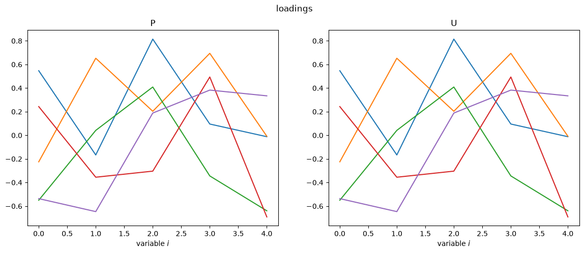
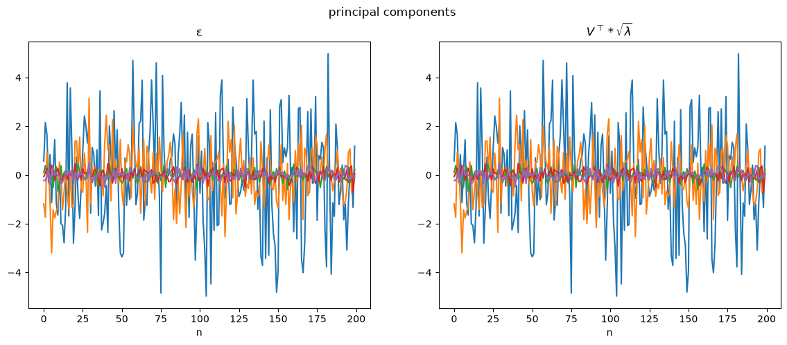
The two algorithms produce the same loadings and the same principal components.
The cumulative fractions of variance explained reveal that two principal components account for almost all of the variation in \(X\), which is consistent with how we generated the data.
print("explained ratio (PCA):", da.explained_ratio_pca)
print("explained ratio (SVD):", da.explained_ratio_svd)
explained ratio (PCA): [0.77 0.98 0.99 0.99 1.  ]
explained ratio (SVD): [0.77 0.98 0.99 0.99 1.  ]
For an example of PCA applied to analyzing the structure of intelligence tests see the lecture Multivariate Normal Distribution.
Look at parts of that lecture that describe and illustrate the classic factor analysis model.
As mentioned earlier, in a sequel to this lecture, VARs and DMDs, we’ll describe how SVD’s provide ways rapidly to compute reduced-order approximations to first-order Vector Autoregressions (VARs).
5.12. Exercises#
Exercise 5.1
In ordinary least squares (OLS), we learn to compute \( \hat{\beta} = (X^\top X)^{-1} X^\top y \), where the matrix \(X\) of regressors has one row for each observation and one column for each regressor.
But the matrix \(X^\top X\) is not invertible (its determinant is zero) when regressors are perfectly collinear or when there are more regressors than observations, so that \(X\) is short and fat and the system \(X \beta = y\) is underdetermined.
And \(X^\top X\) is ill-conditioned when regressors are nearly collinear, meaning that the ratio of its largest to its smallest eigenvalue is very large.
What we can do instead is to use what is called a pseudoinverse \(X^+\) of \(X\) in place of \((X^\top X)^{-1} X^\top\).
Use an SVD of \(X\) to build the pseudoinverse matrix \(X^{+}\) and use it to compute \(\hat{\beta} = X^+ y\).
Show that when \(X\) has linearly independent columns (an over-determined system), \(X^+ = (X^\top X)^{-1} X^\top\), so that \(\hat \beta\) is the usual OLS estimator.
Show that when \(X\) has linearly independent rows (an under-determined system), \(\hat \beta\) solves \(X \beta = y\) exactly and has the smallest norm among all solutions.
Verify these claims numerically for a \(5 \times 8\) matrix \(X\) of random numbers.
Solution
We can use an SVD to compute the pseudoinverse.
Starting from a reduced SVD
in which \(\Sigma\) is the \(p \times p\) diagonal matrix of positive singular values, the pseudoinverse is
Equivalently, in terms of a full SVD, \(X^+ = V \Sigma^+ U^\top\), where the \(n \times m\) matrix \(\Sigma^+\) is formed by transposing \(\Sigma\) and replacing each positive singular value \(\sigma_j\) by \(1/\sigma_j\):
and finally:
When \(X\) has linearly independent columns, \(V\) is a square orthogonal matrix, so
When \(X\) has linearly independent rows, \(U\) is a square orthogonal matrix, so
Every other solution of \(X \beta = y\) has the form \(\beta = \hat \beta + \eta\) with \(X \eta = 0\).
The vector \(\hat \beta = V (\Sigma^{-1} U^\top y)\) lies in the row space of \(X\), which is spanned by the columns of \(V\), while \(\eta\) lies in the null space of \(X\).
These two subspaces are orthogonal, so \(\|\beta\|^2 = \|\hat \beta\|^2 + \|\eta\|^2 \geq \|\hat \beta\|^2\).
Here is a numerical check.
n_obs, k = 5, 8
X = rng.normal(size=(n_obs, k))
y = rng.normal(size=n_obs)

U, σ, VT = np.linalg.svd(X, full_matrices=False)
X_plus = VT.T @ np.diag(1 / σ) @ U.T
β_hat = X_plus @ y

print("X_plus equals np.linalg.pinv(X):", np.allclose(X_plus, np.linalg.pinv(X)))
print("X β_hat = y:                    ", np.allclose(X @ β_hat, y))

# another exact solution: add an element of the null space of X
β_other = β_hat + (np.eye(k) - X_plus @ X) @ rng.normal(size=k)
print("X β_other = y:                  ", np.allclose(X @ β_other, y))
print(f"norms: |β_hat| = {LA.norm(β_hat):.3f}, |β_other| = {LA.norm(β_other):.3f}")

# over-determined case: pseudo-inverse reproduces OLS
X_tall = rng.normal(size=(8, 5))
print("pinv equals (X^T X)^{-1} X^T:   ",
      np.allclose(np.linalg.pinv(X_tall), LA.inv(X_tall.T @ X_tall) @ X_tall.T))
X_plus equals np.linalg.pinv(X): True
X β_hat = y:                     True
X β_other = y:                   True
norms: |β_hat| = 1.099, |β_other| = 1.175
pinv equals (X^T X)^{-1} X^T:    True
Exercise 5.2
This exercise verifies the Eckart-Young theorem numerically.
Construct a \(60 \times 40\) matrix \(X\) equal to a rank-\(4\) matrix plus noise, for example
X = rng.normal(size=(60, 4)) @ rng.normal(size=(4, 40)) + 0.3 * rng.normal(size=(60, 40))
For \(r = 1, 2, 4, 8\)
compute the Eckart-Young approximation \(\hat X_r\) and verify the formulas for \(|| X - \hat X_r ||\) in the spectral, Frobenius, and nuclear norms
compare \(|| X - \hat X_r ||_F\) with \(|| X - Q Q^\top X ||_F\) for \(500\) matrices \(Q\) with \(r\) orthonormal columns that span randomly drawn subspaces (for each \(Q\), \(Q Q^\top X\) is the best approximation of \(X\) whose columns lie in the column space of \(Q\))
Finally, plot the fraction \(\sum_{i \leq r} \sigma_i^2 / \sum_i \sigma_i^2\) against \(r\) and relate it to Step 4 of the PCA recipe above.
Solution
Here is one solution.
m, n = 60, 40
X = rng.normal(size=(m, 4)) @ rng.normal(size=(4, n)) + 0.3 * rng.normal(size=(m, n))
U, σ, VT = np.linalg.svd(X, full_matrices=False)

print(" r   spectral  Frobenius  nuclear   |X - X_r|_F   best random |X - QQ'X|_F")
for r in (1, 2, 4, 8):
    X_r = U[:, :r] @ np.diag(σ[:r]) @ VT[:r, :]
    E = X - X_r
    checks = (np.isclose(LA.norm(E, 2), σ[r]),
              np.isclose(LA.norm(E, 'fro'), np.sqrt(np.sum(σ[r:]**2))),
              np.isclose(LA.norm(E, 'nuc'), np.sum(σ[r:])))
    best_random = np.inf
    for _ in range(500):
        Q = LA.qr(rng.normal(size=(m, r)))[0]
        best_random = min(best_random, LA.norm(X - Q @ Q.T @ X, 'fro'))
    print(f"{r:2d}   {str(checks[0]):8s}  {str(checks[1]):9s}  {str(checks[2]):8s}"
          f"  {LA.norm(E, 'fro'):10.2f}   {best_random:10.2f}")
 r   spectral  Frobenius  nuclear   |X - X_r|_F   best random |X - QQ'X|_F
 1   True      True       True           77.46        96.00
 2   True      True       True           55.16        94.62
 4   True      True       True           13.41        91.33
 8   True      True       True           11.27        84.75
All three error formulas hold, and no randomly drawn rank-\(r\) approximation comes close to the Eckart-Young approximation.
share = np.cumsum(σ**2) / np.sum(σ**2)

fig, ax = plt.subplots()
ax.plot(np.arange(1, len(σ) + 1), share, 'o-')
ax.set_xlabel('$r$')
ax.set_ylabel('fraction of $||X||_F^2$ captured by $\\hat X_r$')
plt.show()
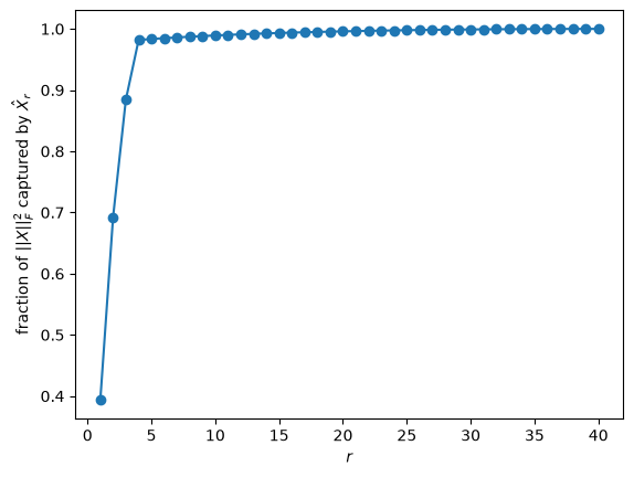
The fraction rises steeply until \(r = 4\), the rank of the signal part of \(X\), and then flattens out.
This fraction is exactly the “fraction of variance retained” that Step 4 of the PCA recipe uses to choose how many principal components to keep, and one minus it is the squared relative Frobenius error of \(\hat X_r\).
Exercise 5.3
This exercise builds a bridge to the sequel VARs and DMDs.
Simulate a tall and skinny time series data set \(\tilde X\) with \(m = 100\) variables and \(61\) periods in which
where \(G\) is a \(100 \times 2\) matrix of standard normal random numbers and \(v_t\) and \(w_{t+1}\) are standard normal random vectors.
Subtract the sample mean of each variable, then use the first \(41\) periods to form \(X = \begin{bmatrix} \tilde X_1 \mid \cdots \mid \tilde X_{40} \end{bmatrix}\) and \(X' = \begin{bmatrix} \tilde X_2 \mid \cdots \mid \tilde X_{41} \end{bmatrix}\).
Compute the least squares estimator \(\hat A = X' X^+\) of the matrix \(A\) in the first-order VAR \(\tilde X_{t+1} = A \tilde X_t + \epsilon_{t+1}\) and verify that it fits perfectly: \(\hat A X = X'\).
Let \(\hat X_2\) be the Eckart-Young rank-\(2\) approximation of \(X\). Verify numerically that \(\hat X_2^+ = V_2 \Sigma_2^{-1} U_2^\top\) and compute the rank-\(2\) estimator \(\hat A_2 = X' \hat X_2^+\).
Let \(F = U_2^\top X\) be the \(2 \times 40\) matrix of the first two principal components of \(X\). Verify that \(\hat A_2 = X' F^\top (F F^\top)^{-1} U_2^\top\), i.e., that \(\hat A_2 \tilde X_t\) equals the fitted value from a regression of \(\tilde X_{t+1}\) on the first two principal components of \(\tilde X_t\).
Use the remaining \(20\) periods to compare one-step-ahead out-of-sample forecast errors \(\|X'_{\rm out} - \check A X_{\rm out}\|_F / \|X'_{\rm out}\|_F\) for \(\check A = \hat A\) and \(\check A = \hat A_2\). Repeat for a few random seeds.
Solution
Here is one solution.
def simulate_tall(m=100, T=61, σ_v=0.5, seed=1):
    rng = np.random.default_rng(seed)
    G = rng.normal(size=(m, 2))
    a = np.array([0.9, 0.6])
    z = np.zeros((2, T))
    for t in range(T - 1):
        z[:, t+1] = a * z[:, t] + rng.normal(size=2)
    X_tilde = G @ z + σ_v * rng.normal(size=(m, T))
    return X_tilde - X_tilde.mean(axis=1, keepdims=True)

def rel_error(A, X, X_prime):
    return LA.norm(X_prime - A @ X) / LA.norm(X_prime)

X_tilde = simulate_tall()
X, X_prime = X_tilde[:, :40], X_tilde[:, 1:41]           # estimation sample
X_out, X_prime_out = X_tilde[:, 40:-1], X_tilde[:, 41:]  # hold-out sample

# 1. minimum-norm least squares estimator
A_hat = X_prime @ np.linalg.pinv(X)
print("A_hat X = X':", np.allclose(A_hat @ X, X_prime))

# 2. pseudo-inverse of the Eckart-Young approximation
U, σ, VT = np.linalg.svd(X, full_matrices=False)
r = 2
U_r, σ_r, V_r = U[:, :r], σ[:r], VT[:r, :].T
X_r = U_r @ np.diag(σ_r) @ V_r.T
X_r_plus = V_r @ np.diag(1 / σ_r) @ U_r.T
print("pinv(X_r) = V_r Σ_r^{-1} U_r^T:", np.allclose(np.linalg.pinv(X_r, rcond=1e-10), X_r_plus))
A_r = X_prime @ X_r_plus

# 3. principal components regression
F = U_r.T @ X
A_pcr = X_prime @ F.T @ LA.inv(F @ F.T) @ U_r.T
print("A_r equals principal components regression:", np.allclose(A_r, A_pcr))

# 4. in-sample and out-of-sample fit
print(f"\nin-sample:     A_hat {rel_error(A_hat, X, X_prime):.3f},  A_r {rel_error(A_r, X, X_prime):.3f}")
print(f"out-of-sample: A_hat {rel_error(A_hat, X_out, X_prime_out):.3f},  A_r {rel_error(A_r, X_out, X_prime_out):.3f}")

print("\nout-of-sample errors for other seeds")
for seed in range(2, 7):
    X_tilde = simulate_tall(seed=seed)
    X, X_prime = X_tilde[:, :40], X_tilde[:, 1:41]
    X_out, X_prime_out = X_tilde[:, 40:-1], X_tilde[:, 41:]
    U, σ, VT = np.linalg.svd(X, full_matrices=False)
    A_r = X_prime @ VT[:r, :].T @ np.diag(1 / σ[:r]) @ U[:, :r].T
    A_hat = X_prime @ np.linalg.pinv(X)
    print(f"seed {seed}:  A_hat {rel_error(A_hat, X_out, X_prime_out):.3f},"
          f"  A_r {rel_error(A_r, X_out, X_prime_out):.3f}")
A_hat X = X': True
pinv(X_r) = V_r Σ_r^{-1} U_r^T: True
A_r equals principal components regression: True

in-sample:     A_hat 0.000,  A_r 0.728
out-of-sample: A_hat 0.999,  A_r 0.757

out-of-sample errors for other seeds
seed 2:  A_hat 0.912,  A_r 0.790
seed 3:  A_hat 0.863,  A_r 0.701
seed 4:  A_hat 0.704,  A_r 0.680
seed 5:  A_hat 0.627,  A_r 0.530
seed 6:  A_hat 0.979,  A_r 0.789
The minimum-norm estimator \(\hat A\) fits the estimation sample perfectly but forecasts poorly out of sample, because the pseudo-inverse \(X^+ = V \Sigma^{-1} U^\top\) puts large weights \(1/\sigma_j\) on directions with small singular values that mostly contain noise.
The rank-\(2\) estimator \(\hat A_2\) discards those directions and forecasts better out of sample.
The estimator \(\hat A_2 = X' \hat X_2^+\) is exactly the estimator that a dynamic mode decomposition computes; the sequel VARs and DMDs studies it in detail.