6. VARs and DMDs#
6.1. Overview#
This lecture applies computational methods that we learned about in the lecture Singular Value Decomposition to
first-order vector autoregressions (VARs)
dynamic mode decompositions (DMDs)
connections between DMDs and first-order VARs
[Sargent et al., 2026] study these connections in detail.
We are especially interested in tall and skinny data sets in which the number of variables \(m\) exceeds the number of time periods \(n\).
Such data sets are common.
For example, [Sargent et al., 2026] study quarterly Consumer Expenditure Survey data on 100 quantiles of each of three cross sections – private income, post-tax-and-transfer income, and consumption – together with aggregate income growth.
That gives them \(m = 301\) variables but only \(n = 133\) quarterly observations.
They use a DMD to estimate a first-order VAR of rank \(3\) for these 301 variables.
Along the way, we’ll learn that
a DMD computes a reduced-rank estimator of the coefficient matrix of a first-order VAR
that estimator is a principal components regression: compress the cross section into a few principal components, then regress next period’s data on them
DMD modes are right eigenvectors of the estimated coefficient matrix
matching left eigenvectors can be computed cheaply, and together with the modes they give an exact modal representation of the estimated VAR that is useful for forecasting and for computing long-run responses
We’ll use the following imports.
import numpy as np
import matplotlib.pyplot as plt
6.2. First-order vector autoregressions#
We want to fit a first-order vector autoregression
where \(\epsilon_{t+1}\) is the time \(t+1\) component of a sequence of IID \(m \times 1\) random vectors with mean vector zero and identity covariance matrix and where the \(m \times 1\) vector \(X_t\) is
Here \(\cdot^\top\) denotes matrix transposition and \(X_{i,t}\) is variable \(i\) at time \(t\).
Equation (6.1) has no constant term.
That is because we assume that each variable has already been transformed – for example, by taking differences, by subtracting a common trend, and by subtracting its time-series mean – so that \(\{X_t\}\) can be regarded as a mean-zero, covariance-stationary process.
For example, [Sargent et al., 2026] subtract a cross-section mean of log private income from every log quantile, use the growth rate of that mean as an additional variable, and then subtract time-series means from all variables.
Our data are organized in an \(m \times (n+1)\) matrix \(\tilde X\)
where for \(t = 1, \ldots, n+1\), the \(m \times 1\) vector \(X_t\) is given by (6.2).
From \(\tilde X\), we form two \(m \times n\) matrices
and
Here \('\) is part of the name of the matrix \(X'\) and does not indicate matrix transposition.
In forming \(X\) and \(X'\), we have in each case dropped a column from \(\tilde X\), the last column in the case of \(X\), and the first column in the case of \(X'\).
We want to estimate a system (6.1) that consists of \(m\) least squares regressions of everything on one lagged value of everything.
The \(i\)th equation of (6.1) is a regression of \(X_{i,t+1}\) on the vector \(X_t\).
So the \(i\)th row of an estimator \(\hat A\) is a \(1 \times m\) vector of regression coefficients of \(X_{i,t+1}\) on \(X_{j,t}, j = 1, \ldots, m\).
A least squares estimator \(\hat A\) solves
where \(\| \cdot \|_F\) denotes the Frobenius norm of a matrix
We denote the rank of \(X\) by \(p \leq \min(m, n)\).
The minimum-norm solution of (6.3) is
where \(X^+\) is the Moore-Penrose pseudo-inverse of \(X\).
Two cases interest us
\(n \gg m\), so that we have many more time series observations \(n\) than variables \(m\)
\(m \gg n\), so that we have many more variables \(m\) than time series observations \(n\)
Short-Fat Case:
When \(n \gg m\) and \(X\) has linearly independent rows, \(X X^\top\) has an inverse and the pseudo-inverse \(X^+\) is
Here \(X^+\) is a right-inverse that verifies \(X X^+ = I_{m \times m}\).
In this case, problem (6.3) has a unique solution and formula (6.4) becomes
This formula for least-squares regression coefficients is widely used in econometrics to estimate vector autoregressions.
The right side of formula (6.5) is proportional to the empirical cross second moment matrix of \(X_{t+1}\) and \(X_t\) times the inverse of the second moment matrix of \(X_t\).
Tall-Skinny Case:
When \(m \gg n\) and \(X\) has linearly independent columns, \(X^\top X\) has an inverse and the pseudo-inverse \(X^+\) is
Here \(X^+\) is a left-inverse that verifies \(X^+ X = I_{n \times n}\).
In this case, formula (6.4) becomes
If we use formula (6.6) to calculate \(\hat A X\) we find that
so that the regression equation fits perfectly.
This is a typical outcome in an underdetermined least-squares model.
In fact, every matrix \(\check A = \hat A + N\) with \(N X = 0\) also fits perfectly, so problem (6.3) has infinitely many solutions.
Formula (6.6) selects the one with the smallest Frobenius norm.
A perfect in-sample fit is a warning sign: with more coefficients than observations, the estimator \(\hat A\) is tracking noise as well as signal.
We’ll respond by constructing a reduced-rank estimator that no longer fits perfectly.
6.2.1. Computing \(X^+\) with an SVD#
An efficient way to compute the pseudo-inverse \(X^+\) is to start with a reduced singular value decomposition
where \(U\) is an \(m \times p\) matrix, \(\Sigma\) is a \(p \times p\) diagonal matrix of positive singular values \(\sigma_1 \geq \sigma_2 \geq \cdots \geq \sigma_p > 0\), and \(V\) is an \(n \times p\) matrix.
As we saw in Singular Value Decomposition, for a reduced SVD
\(U^\top U = I_{p \times p}\) and \(V^\top V = I_{p \times p}\), but
\(U U^\top \neq I_{m \times m}\) unless \(p = m\), and \(V V^\top \neq I_{n \times n}\) unless \(p = n\).
For any rank \(p\), the Moore-Penrose pseudo-inverse of \(X\) is
When \(X\) has linearly independent columns, so that \(p = n\) and \(V\) is a square orthogonal matrix, we can confirm that formula (6.8) agrees with our earlier formula:
where the third line uses \(V^{-1} = V^\top\).
Substituting formula (6.8) into formula (6.4) gives
Formula (6.9) shows a weakness of \(\hat A\).
Small singular values \(\sigma_j\) enter through \(1/\sigma_j\).
So directions in which the data \(X\) vary very little receive very large weights, which amplifies noise.
6.3. A reduced-rank VAR#
A remedy is to keep only the \(r < p\) largest singular values.
Let \(U_r\) be the \(m \times r\) matrix consisting of the first \(r\) columns of \(U\), let \(\Sigma_r\) be the \(r \times r\) upper-left block of \(\Sigma\), and let \(V_r\) be the \(n \times r\) matrix consisting of the first \(r\) columns of \(V\).
Our rank-\(r\) estimator of \(A\) is
The \(m \times m\) matrix \(\hat A_r\) has rank at most \(r\).
Notice that \(V_r \Sigma_r^{-1} U_r^\top\) is the pseudo-inverse of \(\hat X_r = U_r \Sigma_r V_r^\top\), the best rank-\(r\) approximation of \(X\) described by the Eckart-Young theorem in Singular Value Decomposition.
So \(\hat A_r = X' \hat X_r^+\): we obtain the rank-\(r\) estimator by replacing \(X\) with its Eckart-Young approximation in the least squares formula \(\hat A = X' X^+\).
This is the estimator that a dynamic mode decomposition computes.
Dynamic mode decomposition was introduced by [Schmid, 2010].
You can read about it in [Kutz et al., 2016] and [Brunton and Kutz, 2019] (section 7.2).
Associated with \(\hat A_r\) are fitted residuals and their covariance matrix
Thus, our estimated rank-\(r\) VAR is
With \(r < p\), the regression no longer fits perfectly and \(\hat \Omega\) is not zero.
In applications, \(r\) is often very small, e.g., three or fewer.
A common way to choose \(r\) is to plot the singular values \(\sigma_1, \sigma_2, \ldots\) and to truncate where they stop falling rapidly and level off – an “elbow rule.”
[Sargent et al., 2026] used this rule to choose \(r = 3\).
6.3.1. Interpretation as a principal components regression#
We can interpret formula (6.10) statistically.
Define the \(r \times 1\) vector
whose components are the first \(r\) principal components of the cross section \(X_t\) (see the discussion of principal components analysis in Singular Value Decomposition).
Stacking them gives the \(r \times n\) matrix \(F = U_r^\top X = \Sigma_r V_r^\top\).
The least-squares regression of \(X_{t+1}\) on \(f_t\) has coefficient matrix
so that
Similarly, the least-squares regression of \(f_{t+1} = U_r^\top X_{t+1}\) on \(f_t\) has \(r \times r\) coefficient matrix
So \(\tilde A\) is the first-order VAR coefficient matrix for the \(r\) principal components.
Note that \(\tilde A = U_r^\top \hat A_r U_r\).
Thus, a DMD proceeds in two steps:
it compresses the cross section \(X_t\) into \(r\) principal components \(f_t\), using only the variation in \(X\)
it regresses next period’s data \(X_{t+1}\) on those principal components
Statisticians call this a principal components regression.
It resembles the “diffusion index” forecasting method of [Stock and Watson, 2002].
Note
The estimator \(\hat A_r\) is not the matrix of rank \(r\) that minimizes \(\| X' - \check A X \|_F\).
That minimizer is the reduced-rank regression estimator of [Anderson, 1951].
It chooses the \(r\) directions that best predict \(X_{t+1}\), while \(\hat A_r\) uses the \(r\) directions that best describe \(X_t\).
Exercise 6.2 compares the two estimators.
6.4. The DMD algorithm#
Here is the DMD algorithm.
Compute the reduced SVD \(X = U \Sigma V^\top\).
Retain the \(r\) largest singular values to form \(U_r\), \(\Sigma_r\), and \(V_r\).
Form the \(r \times r\) matrix \(\tilde A = U_r^\top X' V_r \Sigma_r^{-1}\) and compute its eigendecomposition
(6.14)#\[ \tilde A W = W \Lambda \]where \(\Lambda\) is a diagonal matrix of eigenvalues \(\lambda_1, \ldots, \lambda_r\) and the columns of \(W\) are corresponding eigenvectors.
Form the \(m \times r\) matrix \(\Phi\) and the \(r \times m\) matrix \(\Psi\)
(6.15)#\[ \Phi = X' V_r \Sigma_r^{-1} W, \qquad \Psi = (W \Lambda)^{-1} U_r^\top \]
The eigenvalues \(\lambda_i\) on the diagonal of \(\Lambda\) are DMD eigenvalues and the columns \(\phi_i\) of \(\Phi\) are DMD modes.
We’ll see below that the rows \(\psi_i\) of \(\Psi\) are matching left eigenvectors.
Notice that the heavy lifting consists of an SVD of the \(m \times n\) matrix \(X\) and an eigendecomposition of the small \(r \times r\) matrix \(\tilde A\).
We never have to form or decompose an \(m \times m\) matrix.
Throughout, we assume that \(\tilde A\) has \(r\) linearly independent eigenvectors and nonzero eigenvalues, which is the generic case.
The matrix \(\tilde A\) is real but not symmetric, so some eigenvalues can come in complex-conjugate pairs.
In that case, the corresponding columns of \(\Phi\) and rows of \(\Psi\) also come in complex-conjugate pairs, while products such as \(\Phi \Lambda^j \Psi\) are real.
For complex matrices, we use \(\cdot^*\) to denote the conjugate transpose.
Note
[Tu et al., 2014] scale the modes differently, defining them as the columns of \(\Phi \Lambda^{-1}\).
With that scaling, the matching left eigenvectors are the rows of \(\Lambda \Psi = W^{-1} U_r^\top\).
Rescaling a mode and its left eigenvector in opposite directions changes none of the formulas below.
6.5. Right eigenvectors: DMD modes#
The following result of [Tu et al., 2014] explains why the columns of \(\Phi\) are called modes.
Proposition 6.1
The columns of \(\Phi\) are eigenvectors of \(\hat A_r\):
Proof. Using formulas (6.10), (6.13), and (6.15),
Equating columns gives \(\hat A_r \phi_i = \lambda_i \phi_i\) for \(i = 1, \ldots, r\).
We can say more.
Write \(\hat A_r = B U_r^\top\), where \(B = X' V_r \Sigma_r^{-1}\) is \(m \times r\).
Because the nonzero eigenvalues of \(B U_r^\top\) coincide with those of \(U_r^\top B = \tilde A\), the eigenvalues of \(\hat A_r\) are \(\lambda_1, \ldots, \lambda_r\) together with \(m - r\) zeros.
So the estimated VAR (6.12) is stable if and only if \(\max_i |\lambda_i| < 1\), a condition we can check with an \(r \times r\) matrix.
(Also see [Brunton and Kutz, 2022], p. 238.)
6.5.1. Projected modes#
[Schmid, 2010] originally worked with the projected modes \(U_r W\) instead of \(\Phi\).
Because \(U_r^\top \Phi = \tilde A W = W \Lambda\), we have
so, up to scale, the projected modes are orthogonal projections of the modes \(\Phi\) onto the column space of \(U_r\).
The projected modes are eigenvectors of \(\hat A_r\) only when \(\Phi = U_r W \Lambda\), that is, when the columns of \(\Phi\) lie in the column space of \(U_r\).
That need not be true, because \(\hat A_r U_r W = \Phi\).
The construction \(\Phi = \hat A_r U_r W\) of [Tu et al., 2014] delivers eigenvectors of \(\hat A_r\) in all cases.
6.6. Left eigenvectors and a modal representation#
Now we come to the rows of \(\Psi\).
Proposition 6.2
Let \(\Psi = (W \Lambda)^{-1} U_r^\top\). Then
\(\Psi \Phi = I_{r \times r}\)
\(\Psi \hat A_r = \Lambda \Psi\), so that the rows of \(\Psi\) are left eigenvectors of \(\hat A_r\)
\(\hat A_r = \Phi \Lambda \Psi = \sum_{i=1}^r \lambda_i \phi_i \psi_i\)
Proof. For the first claim,
For the second claim, since \(U_r^\top \hat A_r = U_r^\top X' V_r \Sigma_r^{-1} U_r^\top = \tilde A U_r^\top\),
For the third claim,
Define the \(r \times 1\) vector of modal coordinates
Computing \(b_t\) requires only the principal components \(f_t = U_r^\top X_t\) and an \(r \times r\) matrix.
Because \(\Psi \Phi = I\), iterating \(\hat A_r = \Phi \Lambda \Psi\) gives
Consequently, the estimated VAR (6.12) implies
and the \(j\)-step-ahead forecast of \(X_{t+j}\) conditional on \(X_t\) is
Each mode \(\phi_i\) contributes a component whose amplitude decays geometrically at rate \(\lambda_i\).
The matrix \(\Phi \Psi\) is an oblique projection onto the column space of \(\Phi\).
It splits \(X_t\) into \(\Phi b_t\) plus a remainder \((I - \Phi \Psi) X_t\) that \(\hat A_r\) sends to zero, because \(\hat A_r (I - \Phi \Psi) = \Phi \Lambda \Psi - \Phi \Lambda \Psi \Phi \Psi = 0\).
6.6.1. A tempting alternative that does not work#
The Moore-Penrose pseudo-inverse \(\Phi^+ = (\Phi^* \Phi)^{-1} \Phi^*\) also satisfies \(\Phi^+ \Phi = I\).
The vector \(\check b_t = \Phi^+ X_t\) is a vector of least squares regression coefficients of \(X_t\) on the columns of \(\Phi\), and \(\Phi \check b_t\) is the orthogonal projection of \(X_t\) onto the column space of \(\Phi\).
That makes \(\check b_t\) a natural descriptive summary of how much each mode is present in \(X_t\).
But in general
so \(\check b_t\) does not evolve according to \(\check b_{t+1} = \Lambda \check b_t\) under the estimated VAR, and \(\Phi \Lambda^j \Phi^+ X_t\) is not the VAR forecast \(\hat A_r^j X_t\).
The reason is that \(\Phi^+\) and \(\Psi\) are both left inverses of \(\Phi\), but their rows span different spaces:
the rows of \(\Phi^+\) span the same space as the rows of \(\Phi^*\)
the rows of \(\Psi\) span the same space as the rows of \(U_r^\top\)
The two left inverses coincide if and only if the column spaces of \(\Phi\) and \(U_r\) are the same.
The column space of \(\Phi\) is the column space of \(X' V_r\), which describes where the data go next period.
The column space of \(U_r\) is spanned by the \(r\) directions in which the current data \(X\) vary most.
These two spaces coincide in special cases, for example when noise-free data are driven by exactly \(r\) factors (see Exercise 6.1), but not in general.
Note
The formula \((W \Lambda)^{-1} U_r^\top X_1\) appears in [Brunton and Kutz, 2022] (p. 240), where it is presented as a computationally cheap approximation to \(\Phi^+ X_1\).
Proposition 6.2 shows that it is exactly the vector of coordinates that is consistent with the dynamics of the estimated VAR.
6.6.2. A state-space representation#
The modal representation lets us write the estimated VAR as a linear state-space system with an \(r \times 1\) state vector.
Define
Then \(X_t = \hat A_r X_{t-1} + \hat a_t = \Phi \Lambda \Psi X_{t-1} + \hat a_t\) and \(\hat x_{t+1} = \Lambda \Psi X_t\) imply
where we have used \(\Psi \Phi = I\).
In representation (6.19)
the state \(\hat x_t\) is the vector of lagged principal components expressed in the eigenvector basis of the principal-component VAR \(\tilde A\)
the transition matrix \(\Lambda\) is diagonal, so the \(r\) components of the state evolve independently, apart from correlated shocks
the columns of \(\Phi\) are loadings of the \(m\) observed variables on the \(r\) components of the state
a single \(m \times 1\) vector of residuals \(\hat a_t\) drives both equations; by the least squares normal equations, it is orthogonal in sample to \(f_{t-1}\) and therefore to \(\hat x_t\)
[Sargent et al., 2026] connect DMDs to linear state-space models of this form.
6.7. Long-run responses#
Modal representation (6.17) also simplifies calculations of long-run responses.
If \(|\lambda_i| < 1\) for all \(i\), then
and
The matrix \(\Lambda (I - \Lambda)^{-1}\) is diagonal with entries \(\lambda_i / (1 - \lambda_i)\).
So long-run responses are dominated by the most persistent modes.
For example, the rank-3 VAR of [Sargent et al., 2026] has DMD eigenvalues \(0.963\), \(0.865\), and \(0.547\), with long-run weights of roughly \(26\), \(6.4\), and \(1.2\).
Formulas like (6.20) appear in additive functionals, which are studied in Additive and Multiplicative Functionals.
Suppose that the first component of \(X_t\) is the growth rate of the logarithm \(Y_t\) of some aggregate, measured as a deviation from its mean \(\nu\), so that \(Y_{t+1} - Y_t - \nu = e_1 X_{t+1}\) where \(e_1 = \begin{bmatrix} 1 & 0 & \cdots & 0 \end{bmatrix}\).
If \(X_t\) obeys the VAR (6.12), then \(Y_t\) can be decomposed into a deterministic trend \(t \nu\), a martingale \(\sum_{j=1}^t H \hat a_j\), and a stationary component \(-g X_t\), plus a constant, where
[Sargent et al., 2026] use this decomposition for aggregate income and for all 300 CEX quantiles.
Formula (6.20) implies
so computing \(g\) and \(H\) requires no inversion of an \(m \times m\) matrix.
6.8. A simulated example#
To see these objects at work, we simulate a tall-skinny data set that shares some features with the CEX data of [Sargent et al., 2026].
There are \(m = 300\) cross-section variables, which we can think of as quantiles indexed by \(q \in [0, 1]\), and \(n + 1 = 134\) quarterly observations.
The cross section is driven by three latent factors \(z_t\) that obey a first-order VAR with a diagonal transition matrix
and the observed data are
where \(w_{t+1}\) and \(v_t\) are standard normal random vectors.
The three columns of \(G\) are shaped like a level factor that moves all quantiles together, a slope factor that moves low and high quantiles in opposite directions, and a curvature factor that moves the tails relative to the middle.
Here is code that simulates the data.
def simulate_data(m=300, T=134, D_diag=(0.95, 0.80, 0.50), σ_v=0.5, seed=1234):
    """
    Simulate an m x T data matrix driven by three latent AR(1) factors.
    """
    rng = np.random.default_rng(seed)
    q = np.linspace(0, 1, m)
    G = np.column_stack([np.ones(m),                # level
                         2 * (q - 0.5),             # slope
                         6 * (q - 0.5)**2 - 0.5])   # curvature
    d = np.array(D_diag)
    k = len(d)
    z = np.zeros((k, T))
    z[:, 0] = rng.normal(size=k) / np.sqrt(1 - d**2)
    for t in range(T - 1):
        z[:, t+1] = d * z[:, t] + rng.normal(size=k)
    X_tilde = G @ z + σ_v * rng.normal(size=(m, T))
    return X_tilde, G, z, q

X_tilde, G, z, q = simulate_data()
X_tilde = X_tilde - X_tilde.mean(axis=1, keepdims=True)   # demean each variable
X_tilde.shape
(300, 134)
The next function implements the DMD algorithm.
def dmd(X_tilde, r):
    """
    Rank-r DMD of the m x (n+1) data matrix X_tilde.
    """
    X, X_prime = X_tilde[:, :-1], X_tilde[:, 1:]
    U, σ, Vt = np.linalg.svd(X, full_matrices=False)
    U_r, σ_r, V_r = U[:, :r], σ[:r], Vt[:r, :].T

    B = X_prime @ V_r / σ_r          # X' V_r Σ_r^{-1}
    A_tilde = U_r.T @ B              # r x r VAR for principal components
    λ, W = np.linalg.eig(A_tilde)
    order = np.argsort(-np.abs(λ))   # most persistent modes first
    λ, W = λ[order], W[:, order]

    Φ = B @ W                              # DMD modes (right eigenvectors)
    Ψ = np.linalg.solve(W * λ, U_r.T)      # (W Λ)^{-1} U_r^T (left eigenvectors)
    A_hat = B @ U_r.T                      # rank-r estimator of A
    a_hat = X_prime - A_hat @ X            # residuals
    Ω_hat = a_hat @ a_hat.T / X.shape[1]

    return dict(λ=λ, Φ=Φ, Ψ=Ψ, W=W, A_tilde=A_tilde, A_hat=A_hat,
                Ω_hat=Ω_hat, σ=σ, U_r=U_r)
To choose \(r\), we plot the largest singular values of \(X\).
σ = np.linalg.svd(X_tilde[:, :-1], compute_uv=False)

fig, ax = plt.subplots()
ax.plot(np.arange(1, 21), σ[:20], 'o')
ax.set_xlabel('index $j$')
ax.set_ylabel(r'singular value $\sigma_j$')
plt.show()
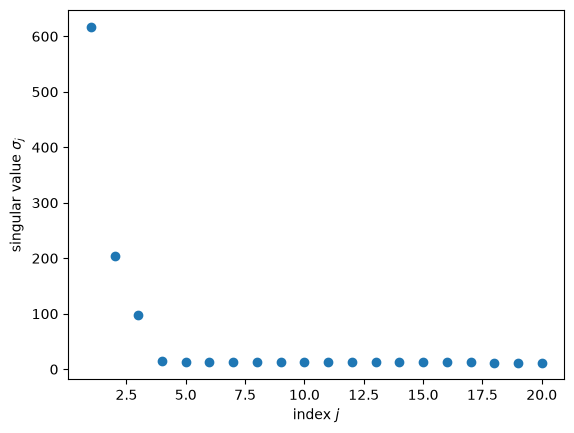
The singular values fall rapidly for \(j = 1, 2, 3\) and then level off, so the elbow rule tells us to set \(r = 3\).
r = 3
res = dmd(X_tilde, r)
λ, Φ, Ψ, A_hat = res['λ'], res['Φ'], res['Ψ'], res['A_hat']

print("DMD eigenvalues:  ", np.round(λ, 3))
print("true eigenvalues: ", np.array([0.95, 0.80, 0.50]))
DMD eigenvalues:   [0.93  0.82  0.337]
true eigenvalues:  [0.95 0.8  0.5 ]
The two most persistent eigenvalues are estimated well.
The least persistent one is biased toward zero.
That is because the data are noisy measurements of the factors, so \(\{X_t\}\) is not exactly a first-order VAR; errors in the principal components \(f_t\) attenuate the estimated coefficients, most visibly for the least persistent mode.
Next we verify Proposition 6.1 and Proposition 6.2, and check whether \(\Phi \Lambda \Phi^+\) equals \(\hat A_r\).
Φ_pinv = np.linalg.pinv(Φ)
rel = lambda M: np.linalg.norm(M) / np.linalg.norm(A_hat)

print("max |A_hat Φ - Φ Λ|        =", np.abs(A_hat @ Φ - Φ * λ).max())
print("max |Ψ Φ - I|              =", np.abs(Ψ @ Φ - np.eye(r)).max())
print("max |Ψ A_hat - Λ Ψ|        =", np.abs(Ψ @ A_hat - λ[:, None] * Ψ).max())
print("relative error, Φ Λ Ψ      =", rel(A_hat - (Φ * λ) @ Ψ))
print("relative error, Φ Λ Φ^+    =", rel(A_hat - (Φ * λ) @ Φ_pinv))
max |A_hat Φ - Φ Λ|        = 1.1796119636642288e-16
max |Ψ Φ - I|              = 1.7763568394002505e-15
max |Ψ A_hat - Λ Ψ|        = 2.7755575615628914e-16
relative error, Φ Λ Ψ      = 1.9407620402191376e-16
relative error, Φ Λ Φ^+    = 0.07337622086364687
The first four numbers are zero up to rounding error, while \(\Phi \Lambda \Phi^+\) misses \(\hat A_r\) by several percent.
Now let’s look at the modes.
Modes are determined only up to scale, so we normalize each mode to have maximum absolute value one and choose its sign to line up with the corresponding column of \(G\), which we normalize in the same way.
def normalize(v):
    return v / np.abs(v).max()

labels = ['level', 'slope', 'curvature']
Φ_real = np.real_if_close(Φ)

fig, axes = plt.subplots(1, 3, figsize=(12, 3.5))
for i, ax in enumerate(axes):
    g_i = normalize(G[:, i])
    φ_i = normalize(Φ_real[:, i])
    φ_i *= np.sign(φ_i @ g_i)
    ax.plot(q, φ_i, lw=2, label=rf'mode $\phi_{i+1}$')
    ax.plot(q, g_i, 'k--', label=f'true {labels[i]} loading')
    ax.set_ylim(-1.1, 1.1)
    ax.set_xlabel('quantile $q$')
    ax.legend()
plt.tight_layout()
plt.show()
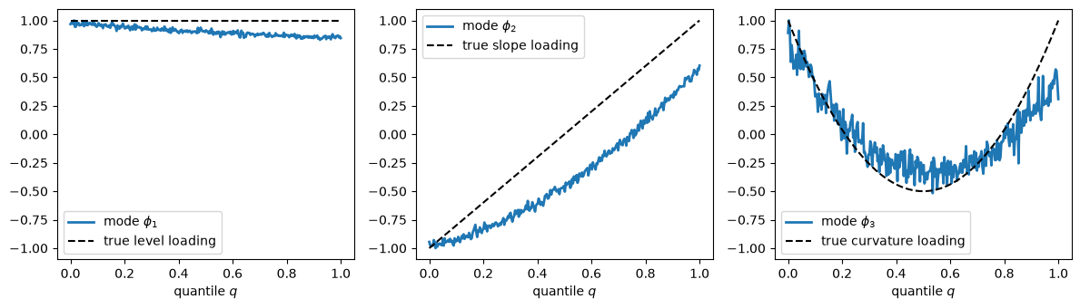
Each mode is close to one of the true loading patterns, but not identical to it.
Because of sampling error, the estimated eigenvectors mix the true factors a little, most visibly for the second mode.
Next we compare the modal coordinates \(b_t = \Psi X_t\) with the true factors \(z_t\), after standardizing both.
b = np.real_if_close(Ψ @ X_tilde)
standardize = lambda x: (x - x.mean()) / x.std()

fig, axes = plt.subplots(3, 1, figsize=(10, 7), sharex=True)
for i, ax in enumerate(axes):
    corr = np.corrcoef(b[i], z[i])[0, 1]
    ax.plot(np.sign(corr) * standardize(b[i]), lw=2, label=rf'$b_{{{i+1},t}}$')
    ax.plot(standardize(z[i]), 'k--', label=rf'$z_{{{i+1},t}}$')
    ax.set_ylabel(f'corr = {abs(corr):.2f}')
    ax.legend(loc='upper right')
axes[-1].set_xlabel('$t$')
plt.tight_layout()
plt.show()
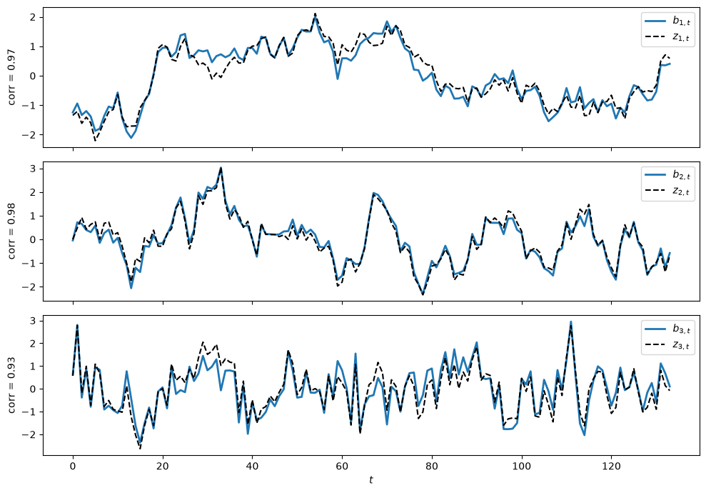
The DMD recovers the latent factors well.
Finally, we compare \(j\)-step-ahead forecasts computed in three ways:
directly from \(\hat A_r^j X_t\)
from the modal representation (6.18) with \(b_t = \Psi X_t\)
from the tempting alternative \(\Phi \Lambda^j \Phi^+ X_t\)
X = X_tilde[:, :-1]
for j in (1, 4, 12):
    direct = np.linalg.matrix_power(A_hat, j) @ X
    via_Ψ = np.real_if_close((Φ * λ**j) @ Ψ @ X)
    via_pinv = np.real_if_close((Φ * λ**j) @ Φ_pinv @ X)
    err = lambda F: np.linalg.norm(F - direct) / np.linalg.norm(direct)
    print(f"j = {j:2d}:  error with Ψ = {err(via_Ψ):.1e},  "
          f"error with Φ^+ = {err(via_pinv):.3f}")
j =  1:  error with Ψ = 1.7e-16,  error with Φ^+ = 0.004
j =  4:  error with Ψ = 2.8e-15,  error with Φ^+ = 0.001
j = 12:  error with Ψ = 1.0e-14,  error with Φ^+ = 0.001
Forecasts built from \(\Psi\) reproduce the VAR forecasts exactly, while those built from \(\Phi^+\) do not.
In this example the forecast discrepancy from using \(\Phi^+\) is small, but, as Exercise 6.1 shows, it grows with the amount of noise in the data.
6.9. Source for some Python code#
You can find a Python implementation of DMD in the PyDMD package.
6.10. Exercises#
Exercise 6.1
In this lecture we saw that \(\Phi^+ = \Psi\) if and only if the column spaces of \(\Phi\) and \(U_r\) are the same.
Simulate data with
simulate_data(σ_v=0.0), so that the data are exact linear combinations of three factors, and compute a rank-3 DMD. Verify numerically that \(\Phi^+ = \Psi\) and that \(\Phi \Lambda \Phi^+ = \hat A_r\).Explain why the column spaces of \(\Phi\) and \(U_r\) coincide in this case.
Repeat part 1 with \(\sigma_v = 0.1, 0.5, 1.0\) and report how far \(\Phi \Lambda \Phi^+\) is from \(\hat A_r\).
Solution
Here is one solution.
for σ_v in (0.0, 0.1, 0.5, 1.0):
    X_sim = simulate_data(σ_v=σ_v)[0]
    X_sim = X_sim - X_sim.mean(axis=1, keepdims=True)
    out = dmd(X_sim, 3)
    Φ_s, Ψ_s, λ_s, A_s = out['Φ'], out['Ψ'], out['λ'], out['A_hat']
    Φ_s_pinv = np.linalg.pinv(Φ_s)
    gap_left = np.linalg.norm(Φ_s_pinv - Ψ_s) / np.linalg.norm(Ψ_s)
    gap_A = np.linalg.norm(A_s - (Φ_s * λ_s) @ Φ_s_pinv) / np.linalg.norm(A_s)
    print(f"σ_v = {σ_v:.1f}:  |Φ^+ - Ψ|/|Ψ| = {gap_left:.1e},  "
          f"|A_hat - Φ Λ Φ^+|/|A_hat| = {gap_A:.1e}")
σ_v = 0.0:  |Φ^+ - Ψ|/|Ψ| = 9.0e-16,  |A_hat - Φ Λ Φ^+|/|A_hat| = 1.1e-15
σ_v = 0.1:  |Φ^+ - Ψ|/|Ψ| = 4.2e-02,  |A_hat - Φ Λ Φ^+|/|A_hat| = 1.5e-02
σ_v = 0.5:  |Φ^+ - Ψ|/|Ψ| = 2.1e-01,  |A_hat - Φ Λ Φ^+|/|A_hat| = 7.3e-02
σ_v = 1.0:  |Φ^+ - Ψ|/|Ψ| = 4.0e-01,  |A_hat - Φ Λ Φ^+|/|A_hat| = 1.4e-01
When \(\sigma_v = 0\), \(X_t = G z_t\) for every \(t\), so every column of both \(X\) and \(X'\) lies in the three-dimensional column space of \(G\).
Because \(X\) has rank three, the column space of \(U_3\) equals the column space of \(G\).
The columns of \(\Phi = X' V_3 \Sigma_3^{-1} W\) are linear combinations of columns of \(X'\), so they also lie in the column space of \(G\).
Since \(\Phi\) has three linearly independent columns, its column space is the column space of \(G\), which is the column space of \(U_3\).
Then the rows of \(\Psi\) lie in the space spanned by the rows of \(\Phi^*\).
So the rows of \(\Psi - \Phi^+\) can be written as \(C \Phi^*\) for some matrix \(C\).
Because \((\Psi - \Phi^+) \Phi = I - I = 0\), we get \(C \Phi^* \Phi = 0\), and since \(\Phi^* \Phi\) is invertible, \(C = 0\).
With measurement noise, \(X'\) has components outside the column space of \(U_3\), the two left inverses differ, and the gap between \(\Phi \Lambda \Phi^+\) and \(\hat A_r\) grows with \(\sigma_v\).
Exercise 6.2
This exercise compares the DMD estimator \(\hat A_r\) with the reduced-rank regression estimator of [Anderson, 1951].
The reduced-rank regression estimator is the rank-\(r\) matrix that minimizes \(\| X' - \check A X \|_F\).
It can be computed as \(\hat A^{RRR}_r = P_r \hat A\), where \(\hat A = X' X^+\) is the minimum-norm least squares estimator and \(P_r = Q_r Q_r^\top\), where the columns of \(Q_r\) are the first \(r\) left singular vectors of the fitted values \(\hat A X\).
Using data from simulate_data(), estimate both rank-3 estimators on the first 100 periods, then
compute the relative in-sample residual norm \(\| X' - \check A X \|_F / \| X' \|_F\) for each estimator
compute the same statistic out of sample, using one-step-ahead forecasts for the remaining periods
repeat for several random seeds and comment on the results
Solution
Here is one solution.
def rrr(X, X_prime, r):
    "Reduced-rank regression estimator of rank r."
    A_full = X_prime @ np.linalg.pinv(X)
    Q = np.linalg.svd(A_full @ X, full_matrices=False)[0][:, :r]
    return Q @ Q.T @ A_full

def rel_resid(A, X, X_prime):
    return np.linalg.norm(X_prime - A @ X) / np.linalg.norm(X_prime)

n_est = 100
print("seed   DMD in   DMD out   RRR in   RRR out")
for seed in range(5):
    X_sim = simulate_data(seed=seed)[0]
    X_sim = X_sim - X_sim.mean(axis=1, keepdims=True)
    X_in, Xp_in = X_sim[:, :n_est-1], X_sim[:, 1:n_est]
    X_out, Xp_out = X_sim[:, n_est-1:-1], X_sim[:, n_est:]

    A_dmd = dmd(X_sim[:, :n_est], 3)['A_hat']
    A_rrr = rrr(X_in, Xp_in, 3)
    print(f"{seed:4d}   {rel_resid(A_dmd, X_in, Xp_in):.3f}    "
          f"{rel_resid(A_dmd, X_out, Xp_out):.3f}     "
          f"{rel_resid(A_rrr, X_in, Xp_in):.3f}    "
          f"{rel_resid(A_rrr, X_out, Xp_out):.3f}")
seed   DMD in   DMD out   RRR in   RRR out
   0   0.515    0.616     0.185    0.709
   1   0.570    0.578     0.228    0.638
   2   0.463    0.788     0.165    0.901
   3   0.429    0.786     0.155    0.946
   4   0.405    0.384     0.155    0.430
By construction, reduced-rank regression has the smaller in-sample residuals.
But in these samples it forecasts worse out of sample than the DMD estimator.
Reduced-rank regression starts from \(\hat A = X' V \Sigma^{-1} U^\top\), which uses all singular values of \(X\), including tiny ones that amplify noise, and then chooses the three directions that best fit \(X'\) in sample.
The DMD estimator instead discards the small singular values before it regresses, which acts as a form of regularization.
Exercise 6.3
Using the rank-3 DMD of the simulated data from the lecture,
verify formula (6.20) numerically by comparing it with a direct computation of \((I - \hat A_r)^{-1}\)
treating the first component of \(X_t\) as the growth-rate variable, compute \(g = e_1 \hat A_r (I - \hat A_r)^{-1}\) both directly and with the modal formula \(g = e_1 \Phi \Lambda (I - \Lambda)^{-1} \Psi\), and report the contribution of each mode to \(g\)
compute the modal formula again with \(\Phi^+\) in place of \(\Psi\) and report how much the answer changes
Solution
For part 1, Proposition 6.2 gives \(\hat A_r = \Phi \Lambda \Psi\) and \(\Psi \Phi = I\).
So \(\hat A_r^2 = \Phi \Lambda (\Psi \Phi) \Lambda \Psi = \Phi \Lambda^2 \Psi\), and induction gives \(\hat A_r^j = \Phi \Lambda^j \Psi\) for \(j \geq 1\).
When \(|\lambda_i| < 1\) for all \(i\),
and since all eigenvalues of \(\hat A_r\) are inside the unit circle, \((I - \hat A_r)^{-1} = I + \sum_{j=1}^\infty \hat A_r^j\).
Here is code for parts 2–4.
m = A_hat.shape[0]
I = np.eye(m)
weights = λ / (1 - λ)

LR_direct = np.linalg.inv(I - A_hat)
LR_modal = np.real_if_close(I + (Φ * weights) @ Ψ)
print("max |direct - modal| for (I - A_hat)^{-1}:",
      np.abs(LR_direct - LR_modal).max())

e1 = np.zeros(m)
e1[0] = 1.0
g_direct = e1 @ A_hat @ LR_direct
g_modal = np.real_if_close(e1 @ (Φ * weights) @ Ψ)
print("max |g_direct - g_modal|:", np.abs(g_direct - g_modal).max())

print("\nlong-run weights λ/(1-λ):", np.round(weights.real, 2))
for i in range(r):
    g_i = np.real_if_close(Φ[0, i] * weights[i] * Ψ[i, :])
    share = np.linalg.norm(g_i) / np.linalg.norm(g_direct)
    print(f"mode {i+1}: |contribution to g| / |g| = {share:.2f}")

g_pinv = np.real_if_close(e1 @ (Φ * weights) @ Φ_pinv)
print("\nrelative error in g using Φ^+:",
      np.linalg.norm(g_pinv - g_direct) / np.linalg.norm(g_direct))
max |direct - modal| for (I - A_hat)^{-1}: 1.457167719820518e-15
max |g_direct - g_modal|: 1.3183898417423734e-15

long-run weights λ/(1-λ): [13.37  4.57  0.51]
mode 1: |contribution to g| / |g| = 1.29
mode 2: |contribution to g| / |g| = 0.66
mode 3: |contribution to g| / |g| = 0.10

relative error in g using Φ^+: 0.026761234549937188
The modal formula reproduces the direct computation up to rounding error, and requires only \(r \times r\) operations beyond forming \(\Phi\) and \(\Psi\).
The most persistent mode, with the largest weight \(\lambda_i/(1-\lambda_i)\), contributes the most to \(g\).
The ratios need not sum to one, and one can exceed one, because contributions of different modes partially offset each other.
Replacing \(\Psi\) by \(\Phi^+\) gives a different, incorrect answer.